Methods to Cope with Lacking Knowledge Utilizing Interpolation Methods in Pandas

Picture by Writer | DALLE-3 & Canva

Lacking values in real-world datasets are a typical drawback. This may happen for numerous causes, reminiscent of missed observations, knowledge transmission errors, sensor malfunctions, and so on. We can’t merely ignore them as they will skew the outcomes of our fashions. We should take away them from our evaluation or deal with them so our dataset is full. Eradicating these values will result in info loss, which we don’t desire. So scientists devised numerous methods to deal with these lacking values, like imputation and interpolation. Individuals usually confuse these two strategies; imputation is a extra widespread time period recognized to newbies. Earlier than we proceed additional, let me draw a transparent boundary between these two strategies.

Imputation is principally filling the lacking values with statistical measures like imply, median, or mode. It’s fairly easy, but it surely doesn’t keep in mind the pattern of the dataset. Nevertheless, interpolation estimates the worth of lacking values based mostly on the encircling developments and patterns. This method is extra possible to make use of when your lacking values will not be scattered an excessive amount of.

Now that we all know the distinction between these strategies, let’s talk about a number of the interpolation strategies obtainable in Pandas, then I’ll stroll you thru an instance. After which I’ll share some suggestions that can assist you select the fitting interpolation approach.

Kinds of Interpolation Strategies in Pandas

Pandas presents numerous interpolation strategies (‘linear’, ‘time’, ‘index’, ‘values’, ‘pad’, ‘nearest’, ‘zero’, ‘slinear’, ‘quadratic’, ‘cubic’, ‘barycentric’, ‘krogh’, ‘polynomial’, ‘spline’, ‘piecewise_polynomial’, ‘from_derivatives’, ‘pchip’, ‘akima’, ‘cubicspline’) that you may entry utilizing the interpolate() operate. The syntax of this technique is as follows:

DataFrame.interpolate(technique='linear', **kwargs, axis=0, restrict=None, inplace=False, limit_direction=None, limit_area=None, downcast=_NoDefault.no_default, **kwargs)

I do know these are plenty of strategies, and I don’t need to overwhelm you. So, we’ll talk about a couple of of them which might be generally used:

• Linear Interpolation: That is the default technique, which is computationally quick and easy. It connects the recognized knowledge factors by drawing a straight line, and this line is used to estimate the lacking values.
• Time Interpolation: Time-based interpolation is helpful when your knowledge isn’t evenly spaced when it comes to place however is linearly distributed over time. For this, your index must be a datetime index, and it fills within the lacking values by contemplating the time intervals between the info factors.
• Index Interpolation: That is just like time interpolation, the place it makes use of the index worth to calculate the lacking values. Nevertheless, right here it doesn’t have to be a datetime index however must convey some significant info like temperature, distance, and so on.
• Pad (Ahead Fill) and Backward Fill Technique: This refers to copying the already existent worth to fill within the lacking worth. If the course of propagation is ahead, it would ahead fill the final legitimate statement. If it is backward, it makes use of the subsequent legitimate statement.
• Nearest Interpolation: Because the title suggests, it makes use of the native variations within the knowledge to fill within the values. No matter worth is nearest to the lacking one shall be used to fill it in.
• Polynomial Interpolation: We all know that real-world datasets are primarily non-linear. So this operate suits a polynomial operate to the info factors to estimate the lacking worth. Additionally, you will have to specify the order for this (e.g., order=2 for quadratic).
• Spline Interpolation: Don’t be intimidated by the advanced title. A spline curve is fashioned utilizing piecewise polynomial features to attach the info factors, leading to a remaining easy curve. You’ll notice that the interpolate operate additionally has piecewise_polynomial as a separate technique. The distinction between the 2 is that the latter doesn’t guarantee continuity of the derivatives on the boundaries, which means it may take extra abrupt modifications.

Sufficient idea; let’s use the Airline Passengers dataset, which accommodates month-to-month passenger knowledge from 1949 to 1960 to see how interpolation works.

Code Implementation: Airline Passenger Dataset

We are going to introduce some lacking values within the Airline Passenger Dataset after which interpolate them utilizing one of many above strategies.

Step 1: Making Imports & Loading Dataset

Import the essential libraries as talked about under and cargo the CSV file of this dataset right into a DataFrame utilizing the pd.read_csv operate.

import pandas as pd
import numpy as np
import matplotlib.pyplot as plt

# Load the dataset
url = "https://uncooked.githubusercontent.com/jbrownlee/Datasets/grasp/airline-passengers.csv"
df = pd.read_csv(url, index_col="Month", parse_dates=['Month'])

parse_dates will convert the ‘Month’ column to a datetime object, and index_col units it because the DataFrame’s index.

Step 2: Introduce Lacking Values

Now, we’ll randomly choose 15 completely different situations and mark the ‘Passengers’ column as np.nan, representing the lacking values.

# Introduce lacking values
np.random.seed(0)
missing_idx = np.random.alternative(df.index, measurement=15, substitute=False)
df.loc[missing_idx, 'Passengers'] = np.nan

Step 3: Plotting Knowledge with Lacking Values

We are going to use Matplotlib to visualise how our knowledge takes care of introducing 15 lacking values.

# Plot the info with lacking values
plt.determine(figsize=(10,6))
plt.plot(df.index, df['Passengers'], label="Authentic Knowledge", linestyle="-", marker="o")
plt.legend()
plt.title('Airline Passengers with Lacking Values')
plt.xlabel('Month')
plt.ylabel('Passengers')
plt.present()

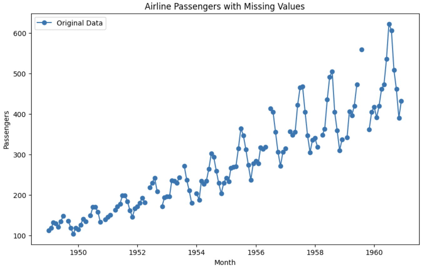
Graph of authentic dataset

You’ll be able to see that the graph is break up in between, displaying the absence of values at these areas.

Step 4: Utilizing Interpolation

Although I’ll share some suggestions later that can assist you choose the fitting interpolation approach, let’s concentrate on this dataset. We all know that it’s time-series knowledge, however because the pattern doesn’t appear to be linear, easy time-based interpolation that follows a linear pattern doesn’t match properly right here. We are able to observe some patterns and oscillations together with linear developments inside a small neighborhood solely. Contemplating these elements, spline interpolation will work properly right here. So, let’s apply that and examine how the visualization seems after interpolating the lacking values.

# Use spline interpolation to fill in lacking values
df_interpolated = df.interpolate(technique='spline', order=3)

# Plot the interpolated knowledge
plt.determine(figsize=(10,6))
plt.plot(df_interpolated.index, df_interpolated['Passengers'], label="Spline Interpolation")
plt.plot(df.index, df['Passengers'], label="Authentic Knowledge", alpha=0.5)
plt.scatter(missing_idx, df_interpolated.loc[missing_idx, 'Passengers'], label="Interpolated Values", shade="inexperienced")
plt.legend()
plt.title('Airline Passengers with Spline Interpolation')
plt.xlabel('Month')
plt.ylabel('Passengers')
plt.present()

Graph after interpolation

We are able to see from the graph that the interpolated values full the info factors and likewise protect the sample. It will possibly now be used for additional evaluation or forecasting.

Suggestions for Selecting the Interpolation Technique

This bonus a part of the article focuses on some suggestions:

1. Visualize your knowledge to grasp its distribution and sample. If the info is evenly spaced and/or the lacking values are randomly distributed, easy interpolation strategies will work properly.
2. In the event you observe developments or seasonality in your time collection knowledge, utilizing spline or polynomial interpolation is healthier to protect these developments whereas filling within the lacking values, as demonstrated within the instance above.
3. Greater-degree polynomials can match extra flexibly however are vulnerable to overfitting. Maintain the diploma low to keep away from unreasonable shapes.
4. For erratically spaced values, use indexed-based strategies like index, and time to fill gaps with out distorting the dimensions. It’s also possible to use backfill or forward-fill right here.
5. In case your values don’t change often or comply with a sample of rising and falling, utilizing the closest legitimate worth additionally works properly.
6. Check completely different strategies on a pattern of the info and consider how properly the interpolated values match versus precise knowledge factors.

If you wish to discover different parameters of the `dataframe.interpolate` technique, the Pandas documentation is the very best place to test it out: Pandas Documentation.

Kanwal Mehreen Kanwal is a machine studying engineer and a technical author with a profound ardour for knowledge science and the intersection of AI with drugs. She co-authored the e-book “Maximizing Productiveness with ChatGPT”. As a Google Technology Scholar 2022 for APAC, she champions range and tutorial excellence. She’s additionally acknowledged as a Teradata Range in Tech Scholar, Mitacs Globalink Analysis Scholar, and Harvard WeCode Scholar. Kanwal is an ardent advocate for change, having based FEMCodes to empower ladies in STEM fields.