[ad_1]
Introduction
Throughout one of many cricket matches within the ICC World Cup T20 Championship, Rohit Sharma, Captain of Indian Cricket Crew had applauded Jasprit Bumrah as Genius Bowler. I made a decision to run a experiment and check it out utilizing knowledge obtainable publicly. Regardless that it’s a enjoyable mission, I used to be pleasantly stunned by the outcomes. Allow us to get began.
Drawback Definition
To do knowledge evaluation or constructing fashions, we have to convert enterprise downside into knowledge downside. How will we make our mannequin perceive which means of Genius. Nicely, Genius might be outlined as “Approach over or Head and Shoulders above the remainder”. Can we formulate this as an Anomaly detection downside? Sure.
There are lots of methods to resolve Anomaly detection downside. We’d follow AutoEncoders utilizing PyTorch.
We’d use publicly obtainable T20 Participant Statistics from cricket knowledge R bundle to coach our AutoEncoders mannequin. If AutoEncoders struggles to reconstruct values then Imply Sq. Error (MSE) could be excessive. MSE over a threshold could be an anomaly.
In our case, MSE for Jasprit Bumrah must be sufficiently excessive to be flagged as anomaly or Genius.
Studying Targets
- Grasp the essential structure of AutoEncoders, together with the roles of the encoder and decoder networks.
- Perceive tips on how to make the most of reconstruction error (Imply Squared Error) from AutoEncoders to establish anomalies.
- Study to preprocess knowledge, create datasets, and arrange knowledge loaders for coaching and testing fashions.
- Perceive the method of coaching an AutoEncoders, together with setting hyperparameters, loss capabilities, and optimizers.
- Discover real-world purposes of anomaly detection, resembling buyer administration and fraud detection.
This text was revealed as part of the Knowledge Science Blogathon.
What are AutoEncoders?
AutoEncoders are composed of two networks Encoder and Decoder. Encoder receives D dimensional vector V and encodes right into a vector X of M dimension whereby M < D. Therefore, Encoder compresses our Enter. Decoder decompresses X and tries to recreate V so far as doable. Allow us to name output of Decoder as Z.
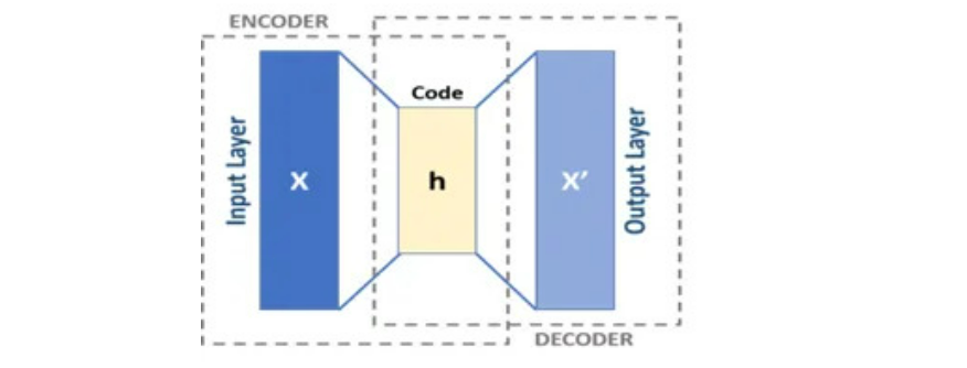
Sometimes, Decoder would capable of recreate V for many of rows i.e for many rows Z could be nearer to V. However for sure rows, Decoder would battle to decode and distinction between Z and V could be large. We’d name these values Anomaly. Anomaly values often have excessive Imply Squared Error or MSE.
Actual World Functions of AutoEncoder
Allow us to now discover actual world purposes of AutoEncoder.
Buyer Administration
Suppose a Group offers with lot of shoppers and has a strategy to label Clients nearly as good or unhealthy, clear or dangerous, rich or non wealthly. Auto Encoder when skilled solely on good or clear or wealthly prospects can decipher sample on these prime or perfect prospects. When a brand new buyer is available in we now have a dependable option to know the way completely different is the brand new buyer from perfect buyer. Chances are you’ll argue that it may be completed manually. People are restricted by quantity of variables and knowledge they will deal with. Machines do not need this limitation.
Fraud Administration
Just like above, if a group has methodology to label transactions as fraudulent or non fraudulent. We will prepare our Autoencoder on Non-Fradulent transactions alone and in manufacturing environments, we now have a dependable mechanism to know the way completely different the brand new transaction from perfect transaction.
Above will not be exhaustive listing of utility of AutoEncoder.
Allow us to now return to our authentic downside.
Knowledge Assortment, Cleansing and Function Engineering
I collected T20 profession statistics knowledge of bowlers right here.
I used R library cricketdata to obtain participant T20 Profession Statistics as python model of the identical will not be obtainable so far as i do know. T20 Statistics doesn’t embody leagues like IPL.
library(cricketdata)
# T20 Profession Knowledge
t20_career <- fetch_cricinfo("T20", "males", "Bowling",'profession')
# T20 Innings Knowledge
t20_innings <- fetch_cricinfo("T20", "males", "Bowling",'innings')
We have to be part of each these datasets and create remaining enter dataset for use for coaching AutoEncoders in Python. Earlier than saving the file to disk we have to think about solely Check Enjoying Nations for our Evaluation.
remaining<-final[Country %in% c('Australia','West Indies','South Africa'
                            ,'Pakistan','Afghanistan','India'
                            ,'Sri Lanka','England','New Zealand'
                            ,'BAN')]
fwrite(remaining,'T20_Stats_Career.txt',sep="|")
We will identify the ultimate dataset as “T20_Stats_Career.txt”.
Now we are going to use Python for our remainder of Evaluation.
import numpy as np
import torch
import torch.optim as optim
import numpy as np
import torch
import torch.optim as optim
import torch.nn as nn
from torch.utils.knowledge import TensorDataset,DataLoader
from sklearn.preprocessing import StandardScaler
import pandas as pd
import matplotlib.pyplot as plt
import seaborn as sns
import random
Now we have imported all needed libraries. We’d now learn Participant’s knowledge.
df = pd.read_csv('T20_Stats_Career.txt',sep='|')
df.head()
First 5 Rows of the dataset is given under:

For each participant, we now have knowledge of Variety of Innings, Overs, Maidens, Runs, Wickets, Common, Economic system and Strike Charge.
Function Engineering
I’ve added two new options:
- Maiden Share: No of Maidens / No of Overs
- Wickets Per Over: No of Wickets / No of Overs
df['Maiden_PCT'] = df['Maidens'] / df['Overs'] * 100
df['Wickets_Per_over'] = df['Wickets'] / df['Overs']
We additionally have to drop Gamers with Variety of Innings lower than 15 in order that we use solely these gamers with adequate match expertise for our Evaluation.
Prepare and Check Dataset
Prepare Dataset: Prepare Datasets would have T20 Statistics of gamers from nationalities aside from India.
Check Dataset: Solely Indian Gamers.
# Create Prepare and Check Dataset
take a look at = df[df['Country'] == 'India']
prepare = df[df['Country'] != 'India']
We use the next options to coach our Mannequin:
- Common
- Economic system
- Strike Charge
- No of 4 Wickets
- No of 5 Wickets
- Maiden Share
- Wickets Per Over
Drop Pointless Options
options = ['Average','Economy','StrikeRate','FourWickets','FiveWickets'
,'Maiden_PCT','Wickets_Per_over']
X_train = prepare[features]
X_test = take a look at[features]
print("Variety of Gamers in Prepare Dataset",X_train.form)
print("Variety of Gamers in Check Dataset",X_test.form)
X_train.head()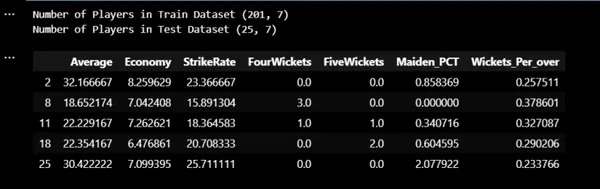
Knowledge Standarization
Now we have prepare and take a look at dataset. Now we have to standardize the information.
sc = StandardScaler()
sc.match(X_train)
X_train = sc.remodel(X_train)
X_test = sc.remodel(X_test)
Mannequin Coaching
We now set acceptable machine and set knowledge loaders with batch measurement of 16.
# Create Tensor Dataset and Dataloders
machine="cuda" if torch.cuda.is_available() else 'cpu'

torch.manual_seed(13)
x_train_tensor = torch.as_tensor(X_train).float().to(machine)
y_train_tensor = torch.as_tensor(X_train).float().to(machine)

x_test_tensor = torch.as_tensor(X_test).float().to(machine)
y_test_tensor = torch.as_tensor(X_test).float().to(machine)

train_dataset = TensorDataset(x_train_tensor,y_train_tensor)
test_dataset = TensorDataset(x_test_tensor,y_test_tensor)

train_loader = DataLoader(dataset=train_dataset,batch_size=16,shuffle=True)
test_loader = DataLoader(dataset=test_dataset,batch_size=16)
We set AutoEncoders Structure as under:
7 ->4->2->4->7.
As we’re coping with very much less knowledge we might construct a easy mannequin.
We use Studying Charge as 0.001 and Adam as Optimizer.
# AutoEncoder Structure

class AutoEncoder(nn.Module):
    def __init__(self):
        tremendous(AutoEncoder,self).__init__()
        self.encoder = nn.Sequential()
        self.encoder.add_module('Hidden1',nn.Linear(7,4))
        self.encoder.add_module('Relu1',nn.ReLU())
        self.encoder.add_module('Hidden2',nn.Linear(4,2))

        self.decoder = nn.Sequential()
        self.decoder.add_module('Hidden3',nn.Linear(2,4))
        self.decoder.add_module('Relu2',nn.ReLU())
        self.decoder.add_module('Hidden4',nn.Linear(4,7))

    def ahead(self,x):
        encoder = self.encoder(x)
        return self.decoder(encoder)

    # Predict Technique
    def predict(mannequin,x):

        mannequin.eval()
        x_tensor = torch.as_tensor(x).float()
        y_hat = mannequin(x_tensor.to(machine))
        mannequin.prepare()

        return y_hat.detach().cpu().numpy()

    # Plot Losses
     def plot_losses(train_losses,test_losses):
        fig = plt.determine(figsize=(10,4))
        plt.plot(train_losses,label="training_loss",c="b")
        #plt.plot(self.val_losses,label="val loss",c="r")
        if test_loader:
            plt.plot(test_losses,label="take a look at loss",c="r")
        #plt.yscale('log')
        plt.xlabel('Epochs')
        plt.ylabel('Loss')
        plt.legend()
        plt.tight_layout()
        return fig

# Mannequin Loss and Optimizer
lr = 0.001
torch.manual_seed(21)
mannequin = AutoEncoder().to(machine)
optimizer = optim.Adam(mannequin.parameters(),lr = lr)
loss_fn =nn.MSELoss()
We prepare our mannequin for 250 epochs.
num_epochs=250
train_loss=[]
test_loss=[]
seed=42
torch.backends.cudnn.deterministic=True
torch.backends.cudnn.benchmark=False
torch.manual_seed(seed)
np.random.seed(seed)
random.seed(seed)
for epoch in vary(num_epochs):
    mini_batch_train_loss=[]
    mini_batch_test_loss=[]
    for train_batch,y_train in train_loader:
        train_batch =train_batch.to(machine)
        mannequin.prepare()
        yhat = mannequin(train_batch)
        loss = loss_fn(yhat,y_train)
        mini_batch_train_loss.append(loss.cpu().detach().numpy())

        loss.backward()
        optimizer.step()
        optimizer.zero_grad()

    train_epoch_loss = np.imply(mini_batch_train_loss)
    train_loss.append(train_epoch_loss)

    with torch.no_grad():
        for test_batch,y_test in test_loader:
            test_batch = test_batch.to(machine)
            mannequin.eval()
            yhat = mannequin(test_batch)
            loss = loss_fn(yhat,y_test)
            mini_batch_test_loss.append(loss.cpu().detach().numpy())
        test_epoch_loss = np.imply(mini_batch_test_loss)
        test_loss.append(test_epoch_loss)

fig = plot_losses(train_loss,test_loss)
fig.savefig('Train_Test_Loss.png')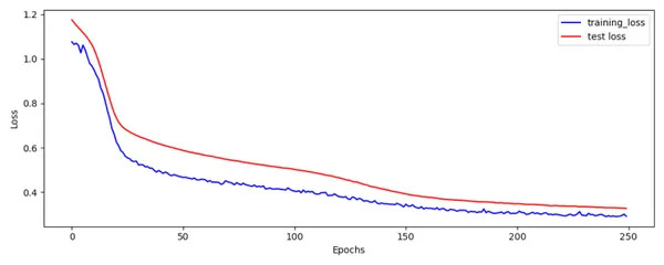
Prepare and Check Loss plot appears OK.
Imply Squared Error (MSE)
Utilizing Predict Operate we will predict for Prepare Dataset. We then compute Imply Squared Error by squaring distinction between Actuals and Predicted. Additionally we are going to compute Z-Rating utilizing imply and normal deviation of MSE.
# Predict Prepare Dataset and get error
train_pred = predict(mannequin,X_train)
print(train_pred.form)
error = np.imply(np.energy(X_train - train_pred,2),axis=1)
print(error.form)
prepare['error'] = error
mean_error = np.imply(prepare['error'])
std_error =np.std(prepare['error'])
prepare['zscore'] = (prepare['error'] - mean_error) / std_error
prepare = prepare.sort_values(by='error').reset_index()
prepare.to_csv('Train_Output.txt',sep="|",index=None)

fig = plt.determine(figsize=(10,4))
plt.title('Distribution of MSE in Prepare Dataset')
prepare['error'].plot(sort='line')
plt.ylabel('MSE')
plt.present()
fig.savefig('Train_MSE.png')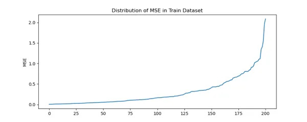
We will infer there’s steep enhance in MSE for sure gamers.
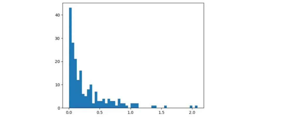
Majority of gamers are inside MSE of 1. Past 1.2 MSE there are solely few gamers.
Prime 3 Gamers within the prepare dataset with highest MSE are:
prepare.tail(3)Please understand that we’re utilizing Tail Operate
We will infer that for some gamers auto encoder struggles to reconstruct authentic values leading to excessive MSE.
By taking a look at above plots, we will set threshold to be 1.2.
I agree that we have to cut up knowledge into prepare and validation and use knowledge of validation dataset to set threshold. However on this case we now have solely 200 rows. We’re compelled to take this method.
Check Dataset – Indian Gamers or Bowlers
Allow us to now compute Imply Squared Error and ZScore for Check Knowledge.
# Predict Check Dataset and get error
test_pred = predict(mannequin,X_test)
test_error = np.imply(np.energy(X_test - test_pred,2),axis=1)
take a look at['error'] = test_error
take a look at['zscore'] = (take a look at['error'] - mean_error) / std_error
take a look at = take a look at.sort_values(by='error').reset_index()
take a look at.to_csv('Test_Output.txt',sep="|",index=None)

fig = plt.determine(figsize=(10,4))
plt.title('Distribution of MSE in Check Dataset')
take a look at['error'].plot(sort='line')
plt.ylabel('MSE')
plt.present()
fig.savefig('Test_MSE.png')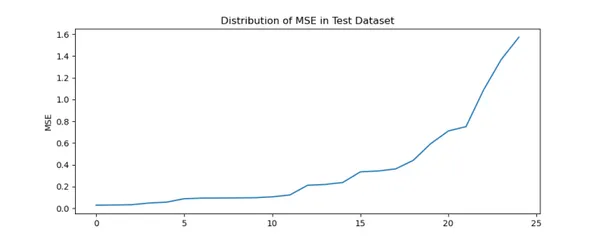
Just like Prepare Dataset there’s steep enhance in MSE for sure Indian Gamers.
take a look at.tail(3)Please understand that we’re utilizing Tail Operate. Therefore Right order is Kuldeep Yadav, JJ Bumrah and Harbhajan Singh.
As in prepare dataset, we create a brand new column named Error in take a look at dataset which has MSE values. Just like Prepare Dataset, Autoencoder is struggling to reconstruct authentic values for some Indian Gamers.
Utilizing Prepare MSE we now have computed imply and normal deviation. For every worth in take a look at dataset we compute Z-Rating as (take a look at error – prepare imply error) / prepare error normal deviation.
We will confirm that Z-Rating for Bumrah is greater than 3 which signifies Anomaly or Genius.
MSE Breakdown or Drill Down
Allow us to now study concerning the MSE breakdown for the gamers.
Jasprit Bumrah
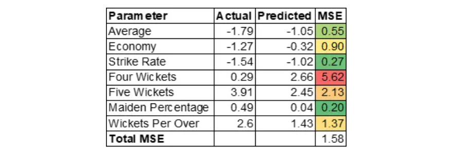
Allow us to now, perceive why MSE is excessive for Jasprit Bumrah. MSE of Jasprit Bumrah is 1.36. Allow us to drill down additional on the MSE at variable stage to know contributing components.
MSE is calculated as (Precise – Predicted) * (Precise – Predicted).
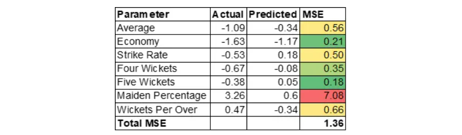
Please word that we’re coping with standardized values. Motive for the excessive MSE is generally contributed by excessive Maiden Share. This implies Bumrah could be an impressive bowler at nineteenth or twentieth over of the innings. Excessive Maiden Share would create stress on batsman which may end up in different bowlers taking wickets within the subsequent over. Please word that variable Maiden Share is was created by Function Engineering.
Kuldeep Yadav
Kuldeep Yadav has uncanny capability of choosing up wickets which will likely be helpful in center overs. Auto Encoder over predicted 4 wickets variable.
Total Statistics of Prime 2 Indian Bowlers
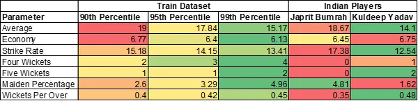
Jasprit Bumrah has 2 variables in additional than ninetieth percentile. Kuldeep Yadav has 4 variables in additional than 99th percentile.
Hope to see Kuldeep Yadav in motion quickly.
You will discover full code right here.
Conclusion
AutoEncoder is a strong instrument in a single’s arsenal for Anomaly Detection however it isn’t the one technique. We will additionally think about using ML algorithms like Isolation Forest or different easier strategies. Coming again to our downside, we will infer that AutoEncoder is ready to accurately establish Anomalies. Hardest half in Anomaly Detection is to persuade stakeholders of the explanations of the Anomaly. Right here we computed drill down of MSE to establish causes for the Anomaly. These insights are as necessary as detecting anomaly itself. Explainable AI is necessary.
Key Takeaways
- We used R Package deal cricketdata to obtain T20 Participant Statistics for take a look at enjoying nations and save the information to disk.
- Do Function Engineering by computing Maiden Share and Wickets Per Over.
- Utilizing PyTorch we might prepare Auto Encoder mannequin for 250 epochs on the Prepare Dataset. We use optimizer as Adam and set studying fee to 0.001.
- Compute Imply Sq. Error by computing distinction between Precise and Prediction in each prepare and take a look at dataset.
- We think about Reconstruction error past a sure threshold as an anomaly. In our case it’s 1.2.
- By taking a look at break up of MSE we will infer that Bumrah excels in bowling Maidens which is gold in T20.
Regularly Requested Questions
A. Sure we will use ML Strategies like Isolation Forest or different Easier strategies to resolve this downside. I’ve used AutoEncoder only for Illustration.
A. Sure, output is completely different when skilled utilizing completely different seeds as knowledge is small.Essential motive of this weblog is to show utility of AutoEncoder and the way it may be used for producing insights to help choice making.
A. Coaching time is lower than a Minute.
A. Deep Studying Framework mustn’t matter. All of it will depend on the framework one is snug with.
The media proven on this article will not be owned by Analytics Vidhya and is used on the Writer’s discretion.
Knowledge Fanatic. Like to bridge hole between knowledge and technique and work on something in between which incorporates knowledge science.
[ad_2]