What’s Conditional Formatting in Excel?

Introduction

Conditional Formatting in Excel is greater than only a function—it’s a strong device reworking the way you work together with information. Whether or not you’re managing a easy funds or analyzing complicated datasets, Conditional Formatting helps you spotlight vital tendencies, patterns, and outliers with only a few clicks. On this article, we’ll discover how one can make the most of this function to make your information extra visually interesting and informative.

Overview

1. Learn the way Conditional Formatting in Excel turns uncooked information into visible insights, making tendencies and outliers stand out.
2. Uncover methods to use Excel’s Conditional Formatting guidelines to routinely spotlight essential information factors with colours, icons, and information bars.
3. Discover making use of personalized Conditional Formatting utilizing Excel formulation for extra nuanced information evaluation.
4. Use Conditional Formatting to identify high/backside performers shortly and duplicate entries in giant datasets.
5. Achieve sensible tricks to maximize the affect of Conditional Formatting with out overwhelming your spreadsheets.
6. Grasp Conditional Formatting to create visually interesting and informative spreadsheets that talk information tales successfully.

Conditional Formatting: An Overview

At its core, Conditional Formatting permits you to apply particular formatting—comparable to colours, icons, or information bars—to cells primarily based on the values they include. This computerized formatting is triggered by guidelines you outline, making it simple to identify essential information factors or tendencies with out manually sifting by numbers.

Additionally learn: Microsoft Excel for Knowledge Evaluation

Highlighting Cells Based mostly on Worth

One of many easiest but simplest makes use of of Conditional Formatting is highlighting cells primarily based on their worth. As an illustration, if you wish to shortly determine which gross sales figures exceed a sure threshold, conditional formatting may help you. Right here’s how:

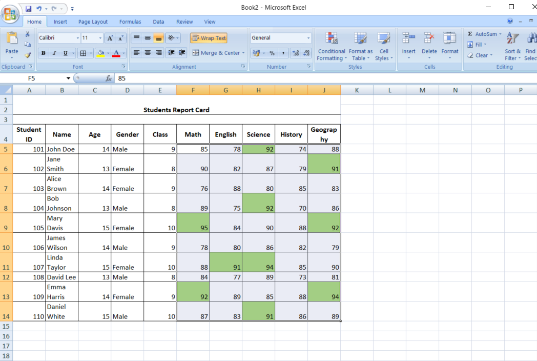
Utilizing Formulation for Customized Formatting

Excel’s flexibility shines if you use formulation to use Conditional Formatting. This enables for extra nuanced and customised guidelines. For instance, you would possibly need to spotlight cells primarily based on a situation that isn’t merely a comparability to a static worth, like flagging gross sales larger than the earlier month’s common.

1. Choose Your Vary: Spotlight the cells you need to format.

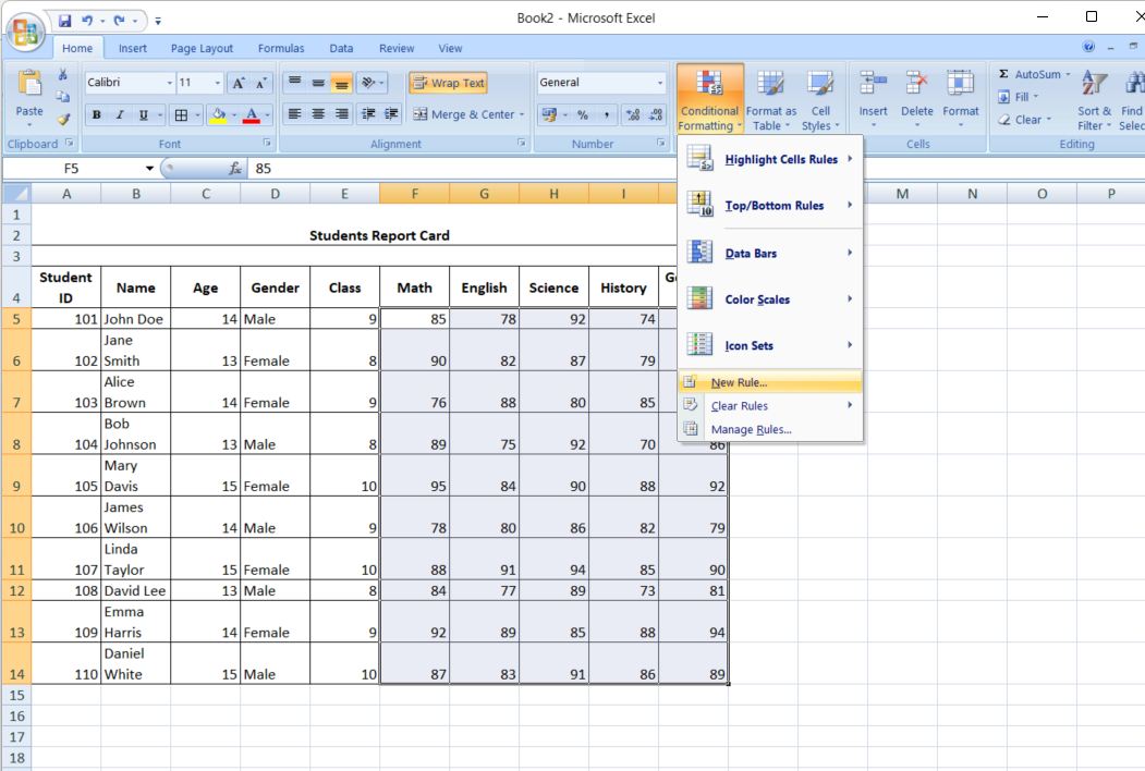
2. Create a New Rule: Below the Conditional Formatting menu, choose “New Rule” and select “Use a formulation to find out which cells to format.”

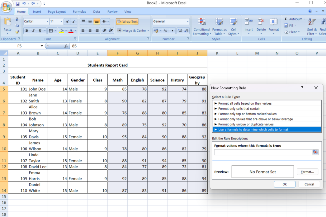
3. Enter the Method: Enter your formulation, which ought to return a TRUE or FALSE final result.

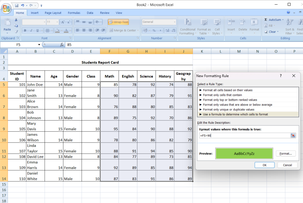
3. Choose a Format: Select the way you need the cells to seem if the situation is met.

4. Apply: Hit OK to see the adjustments in your spreadsheet.

Additionally learn: A Complete Information on Superior Microsoft Excel for Knowledge Evaluation.

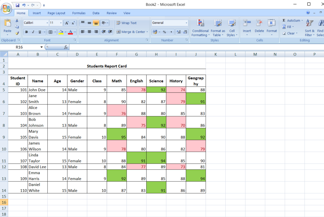
Highlighting Extremes: High/Backside Guidelines

Conditional Formatting also can assist you to give attention to the best and lowest values in a dataset, comparable to figuring out the highest 10 performers or the underside 5 gross sales figures.

• Choose Your Knowledge Vary: Spotlight the related cells.

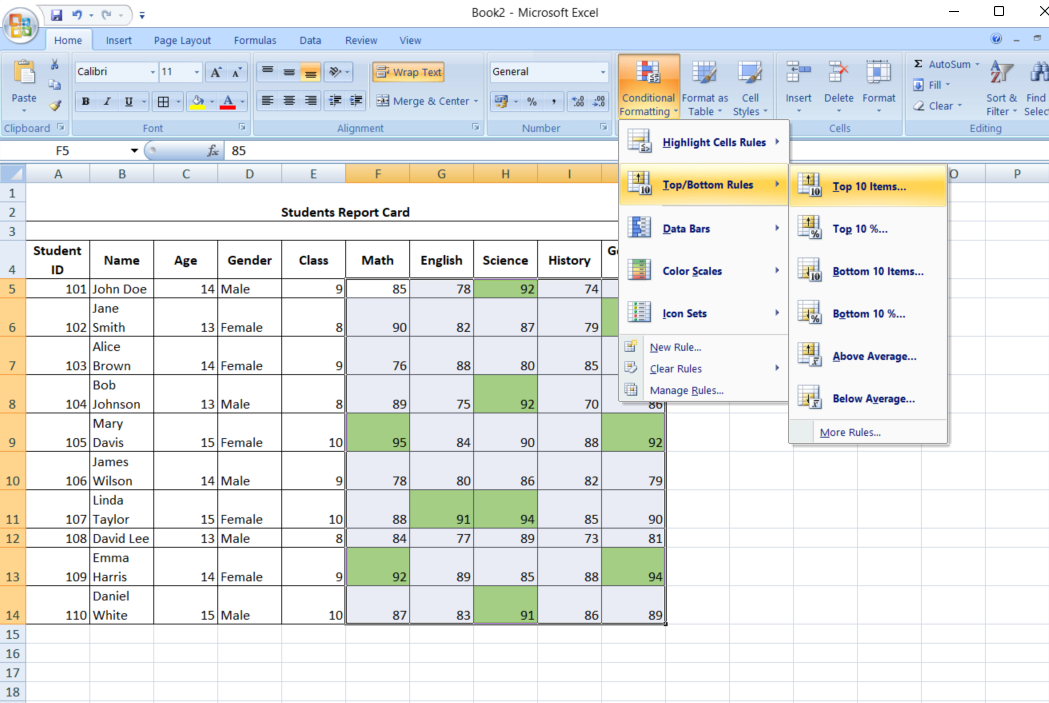
• Entry Conditional Formatting: Navigate to Conditional Formatting > High/Backside Guidelines.
• Set the Parameters: Choose whether or not to spotlight the highest or backside values and specify the variety of gadgets.
• Finalize the Formatting: Choose the specified formatting type and apply the rule.

Equally, figuring out duplicate entries is essential in giant datasets. Conditional Formatting can shortly spotlight duplicates, serving to you keep information accuracy.

• Choose the Vary: Select the cells you need to verify for duplicates.
• Select Duplicate Values Rule: Below the Conditional Formatting menu, choose “Spotlight Cells Guidelines” and “Duplicate Values.”
• Apply Formatting: Decide the formatting type and click on OK.

Ideas for Efficient Use of Conditional Formatting in Excel

Listed below are the information:

1. Begin Easy: Start with fundamental guidelines like highlighting values larger than or lower than a particular quantity. It will assist you to get snug with how Conditional Formatting works.
2. Use Cell References for Flexibility: As a substitute of utilizing static values in your Conditional Formatting guidelines, refer to a different cell. This lets you change the factors by merely updating the reference cell.
3. Leverage Formulation for Customized Guidelines: Excel’s formula-based Conditional Formatting permits you to create extremely personalized guidelines. Be sure that your formulation returns a TRUE or FALSE worth to use the formatting accurately.
4. Mix A number of Guidelines: Don’t hesitate to use a number of Conditional Formatting guidelines to the identical vary of cells. For instance, you should use each Shade Scales and Icon Units to supply totally different layers of knowledge perception.
5. Evaluate and Handle Guidelines Commonly: As you add extra Conditional Formatting, verify and handle your guidelines to keep away from conflicts or overly complicated setups. Use the “Handle Guidelines” choice to edit or delete guidelines as wanted.
6. Prioritize Guidelines: When making use of a number of guidelines, keep in mind that Excel prioritizes them within the order they’re listed. You’ll be able to change the precedence by transferring guidelines up or down within the “Handle Guidelines” dialogue.
7. Use Preview to Your Benefit: Earlier than making use of conditional formatting, use the preview operate to see how your information will look. This helps you tweak the settings for one of the best visible end result.
8. Keep away from Overloading with Formatting: Whereas Conditional Formatting is highly effective, an excessive amount of can overwhelm your spreadsheet and make it tough to learn. Use formatting sparingly to make sure readability.
9. Experiment with Customized Codecs: Excel permits you to create customized formatting kinds (e.g., particular colours or font kinds) in Conditional Formatting. That is significantly helpful for sustaining a constant look throughout your spreadsheets.
10. Clear Formatting When Wanted: In case your information adjustments considerably, clear the previous formatting guidelines to start out contemporary. This prevents outdated guidelines from making use of incorrectly to new information.

Conclusion

Conditional Formatting in Excel isn’t just a helpful function—it’s a game-changer for anybody who works with information. By leveraging this device, you may flip a easy spreadsheet right into a dynamic, visually interesting report highlighting key insights and tendencies at a look. Whether or not you’re an information novice or an skilled analyst, mastering Conditional Formatting will improve your capacity to speak data-driven tales successfully. So, the following time you’re in Excel, don’t simply take a look at the numbers—let Conditional Formatting assist you to see the larger image.

Regularly Requested Questions